池化层

1. 池化层的作用与意义

像素矩阵输入到卷积层，与卷积核进行互相关运算后，由局部感受野提取局部特征（如边缘、纹理等），保留了输入数据的空间结构。但计算机视觉任务的决策基于图像全局，而不是局部特征。

1.1 池化操作的基本类型

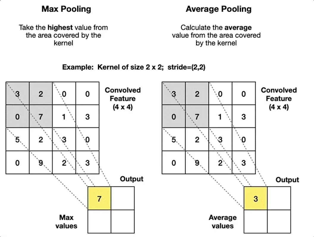
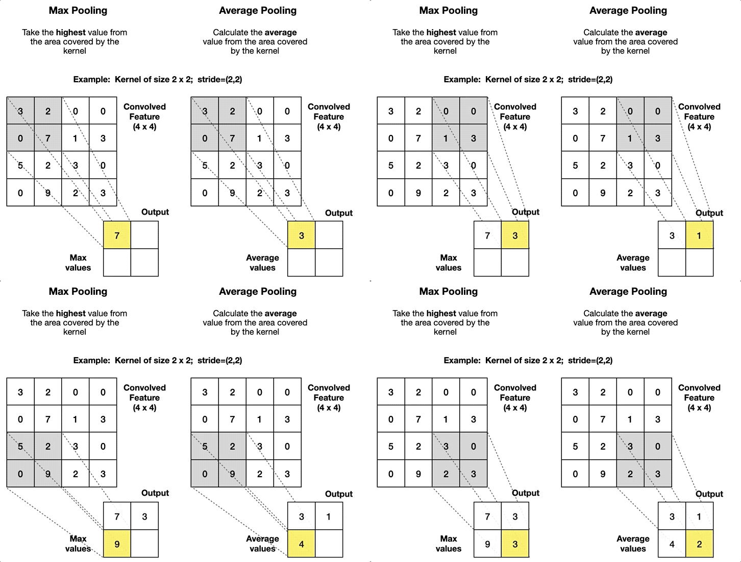
与卷积层的感受野类似，池化层使用池化窗口 (pooling window) 限制降采样过程中区域的大小和形状。

2. 池化层的实现

与卷积层中执行二维互相关运算的函数类似，我们定义 pool2d() 函数实现基本的池化操作：

2.1 基础池化函数实现

from typing import Literal, Tuple
import torch

def pool2d(input2d: torch.Tensor, window: Tuple[int, int], mode: Literal['max', 'avg']) -> torch.Tensor:
    """
    二维池化运算
    
    参数:
        input2d: 输入的二维张量
        window: 池化窗口大小 (height, width)
        mode: 池化模式，'max' 或 'avg'
    
    返回:
        池化后的二维张量
    """
    h_input, w_input = input2d.shape
    h_window, w_window = window

    # 不使用填充时的输出尺寸
    h_output = h_input - h_window + 1
    w_output = w_input - w_window + 1

    output = torch.empty(h_output, w_output)

    # 池化运算
    for h in range(h_output):
        for w in range(w_output):
            window_region = input2d[h:h + h_window, w:w + w_window]
            if mode == 'max':
                output[h, w] = window_region.max()
            elif mode == 'avg':
                output[h, w] = window_region.mean()
            else:
                raise NotImplementedError("只实现了 'max' 和 'avg' 池化")

    return output

# 测试最大池化
input_data = torch.tensor([[0.0, 1.0, 2.0],
                          [3.0, 4.0, 5.0],
                          [6.0, 7.0, 8.0]])

max_result = pool2d(input_data, window=(2, 2), mode='max')
avg_result = pool2d(input_data, window=(2, 2), mode='avg')

print(f'输入数据:\n{input_data}')
print(f'最大池化结果:\n{max_result}')
print(f'平均池化结果:\n{avg_result}')

输入数据:
tensor([[0., 1., 2.],
        [3., 4., 5.],
        [6., 7., 8.]])
最大池化结果:
tensor([[4., 5.],
        [7., 8.]])
平均池化结果:
tensor([[2.0000, 3.0000],
        [5.0000, 6.0000]])

2.2 填充和步幅

与卷积层类似，池化运算前同样支持对特征图边界的填充 (padding)，并通过步幅 (stride) 改变池化窗口移动的步长。

以下使用 PyTorch 中内置的二维最大池化层 nn.MaxPool2d() 演示：

import torch
from torch import nn

# 创建4×4的输入数据
data = torch.arange(16, dtype=torch.float32).reshape(1, 1, 4, 4)

# 不同参数配置的池化层
layer1 = nn.MaxPool2d(kernel_size=3, padding=1, stride=2)
layer2 = nn.MaxPool2d(kernel_size=(2, 3), stride=(2, 3), padding=(0, 1))

# 执行池化操作
result1 = layer1(data)
result2 = layer2(data)

print('原始数据:')
print(data.squeeze())
print(f'\n配置1 - kernel_size=3, padding=1, stride=2:')
print(result1.squeeze())
print(f'\n配置2 - kernel_size=(2,3), stride=(2,3), padding=(0,1):')
print(result2.squeeze())

原始数据:
tensor([[ 0.,  1.,  2.,  3.],
        [ 4.,  5.,  6.,  7.],
        [ 8.,  9., 10., 11.],
        [12., 13., 14., 15.]])

配置1 - kernel_size=3, padding=1, stride=2:
tensor([[ 5.,  7.],
        [13., 15.]])

配置2 - kernel_size=(2,3), stride=(2,3), padding=(0,1):
tensor([[ 5.,  7.],
        [13., 15.]])

3. 多通道池化

与卷积层类似，池化层也需要处理多通道的数据。但与卷积层不同的是：

3.1 多通道池化实现

import torch
from torch import nn

# 创建双通道数据
channel1 = torch.arange(16, dtype=torch.float32).reshape(1, 1, 4, 4)
channel2 = channel1 + 1
multi_channel_data = torch.cat((channel1, channel2), dim=1)

# 定义池化层
pooling_layer = nn.MaxPool2d(kernel_size=3, padding=1, stride=2)
pooling_result = pooling_layer(multi_channel_data)

print('多通道输入数据:')
print('通道1:')
print(multi_channel_data[0, 0])
print('通道2:')
print(multi_channel_data[0, 1])

print('\n池化结果:')
print('输出通道1:')
print(pooling_result[0, 0])
print('输出通道2:')
print(pooling_result[0, 1])

print(f'\n输入形状: {multi_channel_data.shape}')
print(f'输出形状: {pooling_result.shape}')

多通道输入数据:
通道1:
tensor([[ 0.,  1.,  2.,  3.],
        [ 4.,  5.,  6.,  7.],
        [ 8.,  9., 10., 11.],
        [12., 13., 14., 15.]])
通道2:
tensor([[ 1.,  2.,  3.,  4.],
        [ 5.,  6.,  7.,  8.],
        [ 9., 10., 11., 12.],
        [13., 14., 15., 16.]])

池化结果:
输出通道1:
tensor([[ 5.,  7.],
        [13., 15.]])
输出通道2:
tensor([[ 6.,  8.],
        [14., 16.]])

输入形状: torch.Size([1, 2, 4, 4])
输出形状: torch.Size([1, 2, 2, 2])